CHAPTER 12 FIGURES
To see full-size figures, just click the thumbnails. To download
high-resolution PDF versions for printing, please click here.
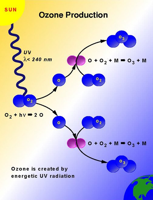
- Figure 12.01
- Schematic diagram of ozone production

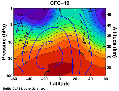
- Figure 12.02
- CFC-12 zonally averaged concentrations as a function of height
with arrows showing stratospheric circulation pattern

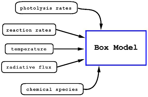
- Figure 12.03
- Schematic diagram of a box model

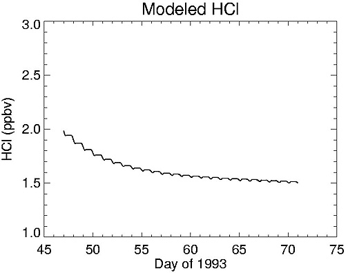
- Figure 12.04
- Modeled HCl concentrations reaching a photochemical
equilibrium state over the course of a 3-week box model run

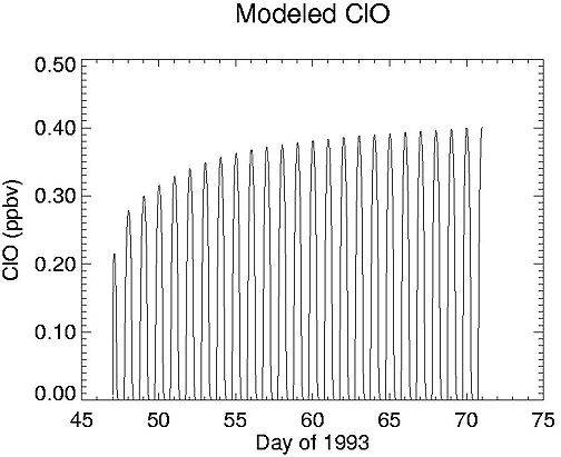
- Figure 12.05
- Modeled ClO concentrations reaching a diurnal cycle
photochemical equilibrium state over the course of a 3-week box
model run
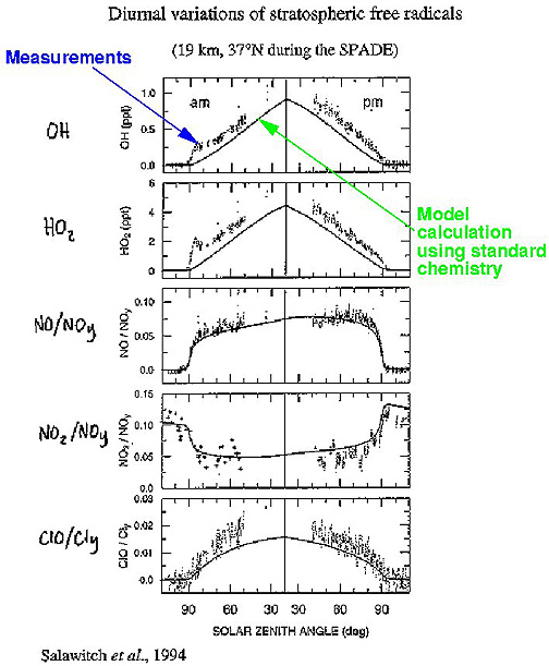
- Figure 12.06
- Comparison of box model and ER-2 suite observations of
stratospheric free radical diurnal variability
- Figure 12.07
- Making an air parcel trajectory map
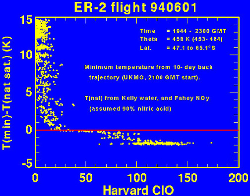
- Figure 12.08
- ER-2 flight data of temperature differences vs ClO
concentrations: minimum temp. based on 10-day back trajectory
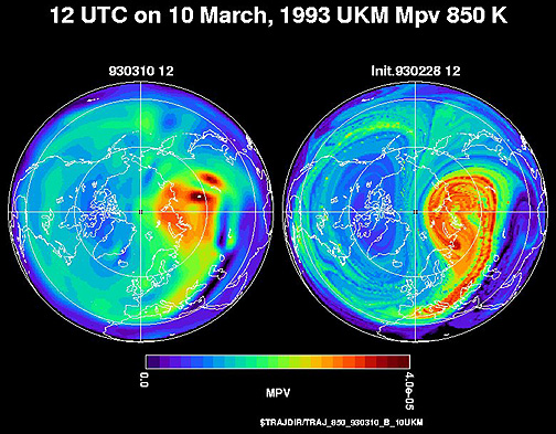
- Figure 12.09
- Evolution of contours of potential vorticity using a 10-day
back trajectory model for March 10, 1993, on 850 K surface
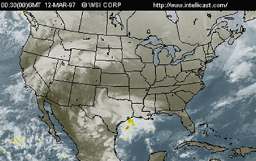
- Figure 12.10
- Satellite picture of cloud distribution over North
America
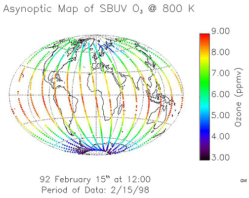
- Figure 12.11
- Map of SBUV-measured individual ozone observations made over
the course of a 24-hr period on February 15, 1992
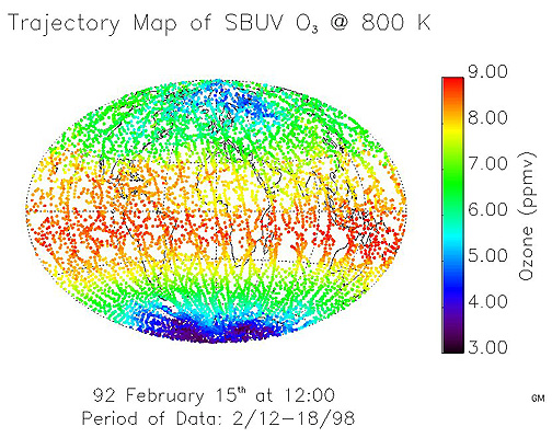
- Figure 12.12
- Map of SBUV-measured ozone observations on February 15, 1992,
run by a trajectory model forward and backward

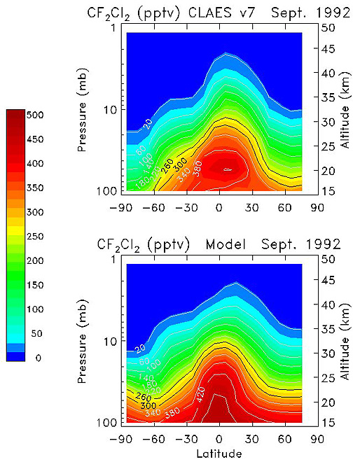
- Figure 12.13
- Comparison of satellite measured CFC-12 zonal mean
distribution with height to GSFC 2-D zonal mean model for
September 1992

- Figure 12.14
- Comparison of satellite measured ClO zonal mean distribution
with height to 2-D zonal mean model for August-October 1992 data:
difference shown in bottom panel as a way of illustrating
overprediction problem
- Figure 12.15
- Comparison of satellite measured ozone zonal mean distribution
with height to 2-Dd zonal mean model for September 1992:
difference shown in bottom panel
- Figure 12.16
- Long-term projections of atmospheric chlorine concentrations
based on each of the international CFC agreements
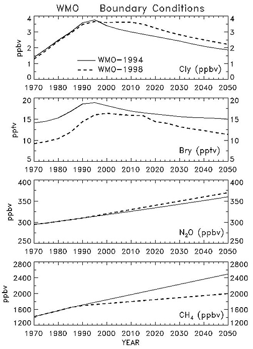
- Figure 12.17
- WMO 1994 and 1998 assessments and long-term forecasts
(1970-2050) for four different constituents important to
stratospheric ozone concentrations
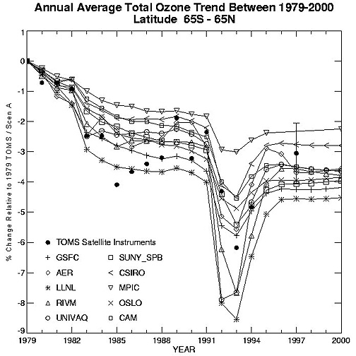
- Figure 12.18
- Annual average ozone trend between 1979-2000 for 65°S to
65°N (global avg.) as predicted by an ensemble of ten 2-D
ozone models: trends compared to 1979-1997 TOMS measured data for
validation
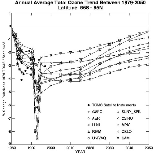
- Figure 12.19
- Annual average ozone trend between 1979-2050 for 65°S to
65°N (global avg.) as predicted by an ensemble of ten 2-D
ozone models: trends compared to 1979-1997 TOMS measured data for
validation
- Figure 12.20
- Percent changes in total ozone from 1979 for 65°S to
65°N (global avg.) based on different input assumptions
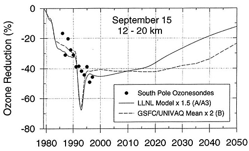
- Figure 12.21
- Percent reduction in ozone column over the South Pole as
predicted by three 2-D models for 1979-2050: comparisons to South
Pole ozonesondes shown for validation